Why waste resources computing deformation on non-deforming regions? Use our method instead.
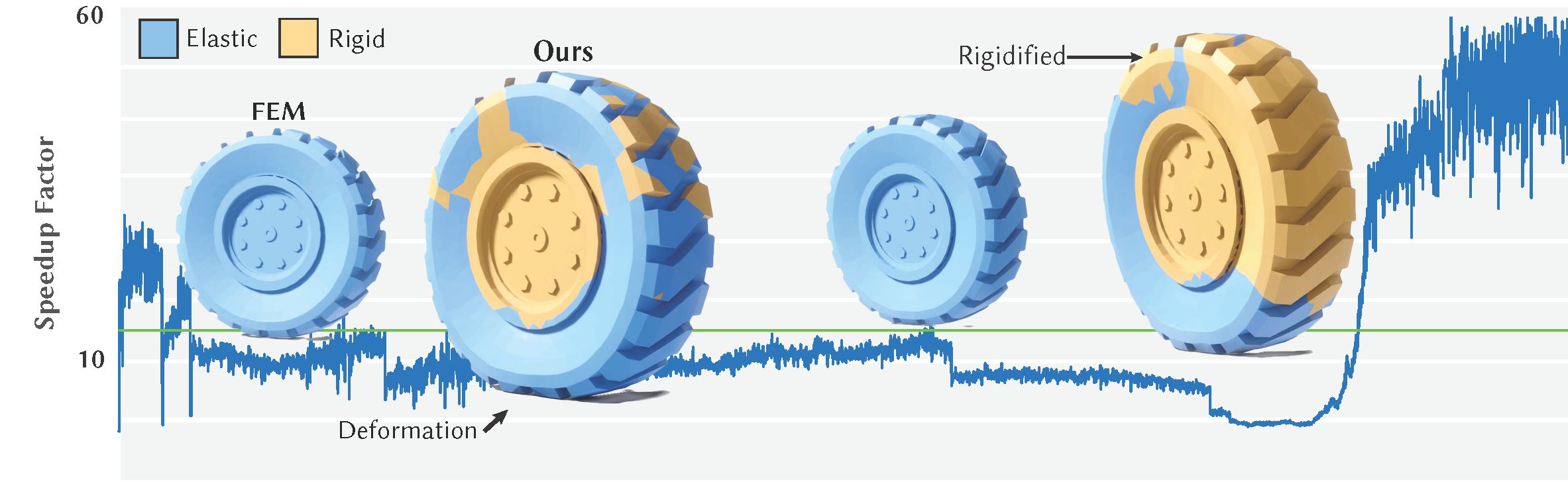
Abstract: We present a method for reducing the computational cost of elastic solid simulation by treating connected sets of non-deforming elements as rigid bodies. Non-deforming elements are identified as those where the strain rate squared Frobenius norm falls below a threshold for several frames. Rigidification uses a breadth first search to identify connected components while avoiding connections that would form hinges between rigid components. Rigid elements become elastic again when their approximate strain velocity rises above a threshold, which is fast to compute using a single iteration of conjugate gradient with a fixed Laplacian-based incomplete Cholesky preconditioner. With rigidification, the system size to solve at each time step can be greatly reduced, and if all elastic element become rigid, it reduces to solving the rigid body system. We demonstrate our results on a variety of 2D and 3D examples, and show that our method is likewise especially beneficial in contact rich examples.
![]()
![]()
![]()
Installation
Full Presentation
Supplemental Video
Authors
Alexandre Mercier-Aubin, Alexander Winter, David I.W. Levin, and Paul G. Kry
Embedded paper
Summarized Version
Here is a summarized version of this paper. The pre-print can be downloaded using the link above.
Mixing Rigids and Elastics
Rigidification
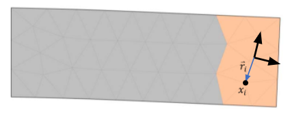
If the rotationally invariant Green strain tensor $E=\frac{1}{2}(F^TF-I)$ remains constant for a period of time, then we allow the element to become rigid.
For time step $k$, we compute the strain rate using finite difference
We use an adjacency graph for tetrahedral elements with shared faces (or with shared edges for triangle elements in 2D simulations). Each connected component forms a rigid body in our simulation.
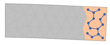
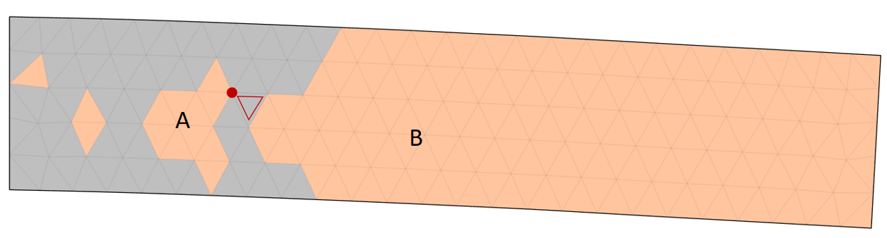
There are two possibilities to handle the case where rigid bodies share a vertex. One can add hinge constraints; this will slow down the time integration. We instead choose to make our BFS greedy, the first rigid element to touch a vertex (edge in 3D) claims it. Note that when this case happens, the neighboring elements often rigidify on the next frame.
Elastification
Consider an oracle that determines which elements should elastify. We propose a single preconditioned conjugate gradient iteration to approximate the strain rate, which we compare to an elastification threshold. The propagation of the information is critical to generate good elastification behavior. Preconditioning is essential, otherwise each iteration only propagates information between neighbours following the sparsity structure of the system.
Incomplete Cholesky factorization is a good choice because the forward and backward substitution provides an excellent opportunity for an impulse at one vertex to influence $\dot{x}_\text{approx}$ at distant vertices, even with only one iteration of conjugate gradient
Local rigidification
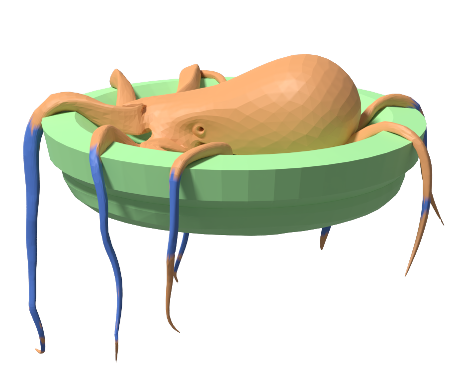
Our technique works like sleeping on static bodies, yet it really shines in scenes with local deformation. This effectively reduces the size of the system to solve from $3n$ vertices to exactly 6 degrees of freedom for a rigidified chunk of the models. As the time to solve is dependent on the degrees of freedom in the full system, this significantly reduces the computation time of the simulation.
See our paper for more details and results
click here for the code if you missed the two github buttons
Bibtex
@InProceedings{ARES,
author = {Mercier-Aubin, Alexandre and Kry, Paul G. and Winter, Alexandre and Levin, David I. W.},
title = {Adaptive Rigidification of Elastic Solids},
year = {2022},
issue_date = {July 2022},
publisher = {Association for Computing Machinery},
address = {New York, NY, USA},
volume = {41},
number = {4},
issn = {0730-0301},
url = {https://dl.acm.org/doi/abs/10.1145/3528223.3530124},
doi = {10.1145/3528223.3530124},
abstract = {We present a method for reducing the computational cost of elastic solid simulation by treating connected sets of non-deforming elements as rigid bodies. Non-deforming elements are identified as those where the strain rate squared Frobenius norm falls below a threshold for several frames. Rigidification uses a breadth first search to identify connected components while avoiding connections that would form hinges between rigid components. Rigid elements become elastic again when their approximate strain velocity rises above a threshold, which is fast to compute using a single iteration of conjugate gradient with a fixed Laplacian-based incomplete Cholesky preconditioner. With rigidification, the system size to solve at each time step can be greatly reduced, and if all elastic element become rigid, it reduces to solving the rigid body system. We demonstrate our results on a variety of 2D and 3D examples, and show that our method is likewise especially beneficial in contact rich examples.},
journal = {ACM Trans. Graph.},
month = {jul},
articleno = {71},
numpages = {11},
keywords = {physics simulation, adaptive, rigid bodies, finite element method}
}